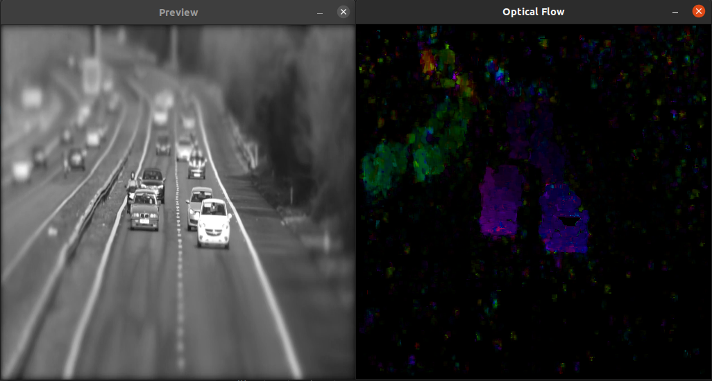
Optical flow is a method in computer vision to estimate the apparent velocity of pixels in an image by measuring the shift of its brightness distribution between consecutive frames. We can leverage this information for a variety of applications, like object tracking or visual odometry. In this project, I wrote the functions for the Lukas-Kanade method from scratch to gain a better understanding of this algorithm as well as to improve my skills in C++.
Image as a function
We can imagine an image as a surface in 3D, where the x and y axes correspond to the pixels in the image, and the z-axis corresponds to the image brightness (1-channel image). We can then imagine the gradient of this surface with respect to x and y as being the shift in the image brightness as we move along either of the axes. We cannot compute these derivatives directly, but we can approximate them using finite differences, which is the derivative’s discrete counterpart.
When we have two consecutive image frames, we can compute the derivative of the image with respect to time, again approximating with finite differences.
Tying everything together
We are looking to compute the velocities Vx and Vy, which represent the image pixel velocities in the x and y axes, respectively. The optical flow equation states the following:
Intuitively, we are trying to find the velocity vector for windows of pixels in the image where the shift in brightness matches that of what we have observed along the time axis. For a given window of pixels, we can evaluate the solution of this overdetermined system using least squares estimation.